Project 2: Gradient Domain Cloning

CS 6501 - Computational Photography

Due: Mon, Oct 7 (11:59 PM)

This project has one required part and one optional part. In the required part, you will implement gradient-domain compositing. In the optional part, you can implement seam carving for extra credit.

Required Part: Gradient Domain Cloning

The human visual system is quite sensitive to gradients: it tends to ignore small gradients and pick up large gradients. This is exploited the seam carving part of the assignment also. As discussed in Lecture 5, researchers have developed a dual representation of images called the gradient domain which is just the gradient or x and y derivatives of the input image (in each color channel). One can modify gradients however one wishes, apply boundary conditions, and then "integrate" using a linear solver to go back to color domain. This allows for many applications such as the artistic depiction in GradientShop.

Your assignment is to implement the gradient domain cloning application of Perez et al 2003. Your algorithm should take as input a background image B, a foreground image F and a matte image M which is either black to indicate selection of the background or white to indicate foreground. First as a sanity check you can try pasting the foreground on top of the background naively:

I_naive = B + M(F - B)
A naive cloning result is shown in Figure 3 of the paper (two foregrounds have been pasted, one after the other):

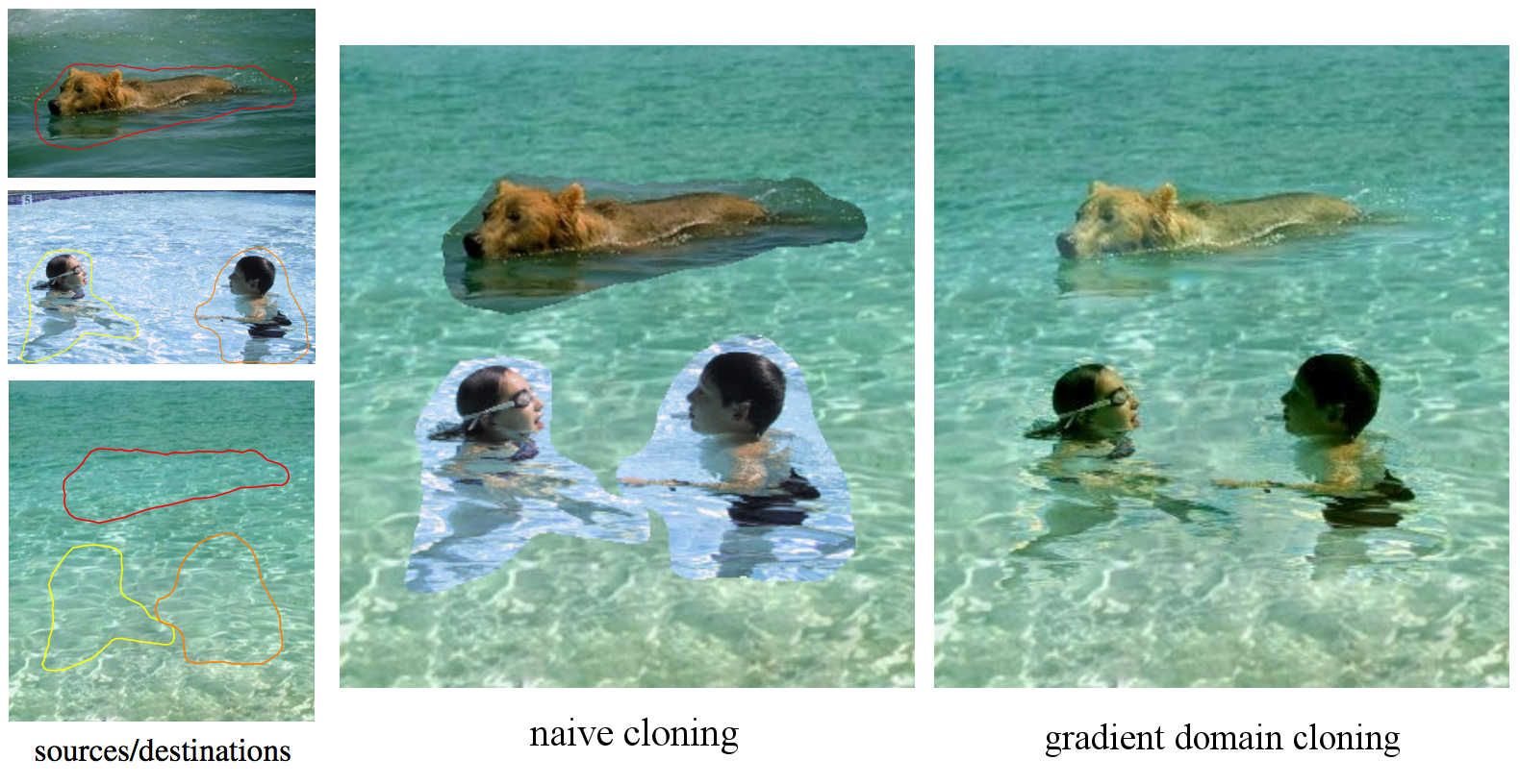
Your goal is to compute the gradient domain cloning result shown at right. This is done by solving a differential equation that tries to match the gradients of the result R to the foreground image F while using a boundary condition given by the background image B along the boundary of the matte. The paper solves for each color channel independently, so you can simply loop over each of the RGB channels and solve for each independently. We now assume that we are working within one channel.

You can implement gradient domain cloning by following the paper's derivation. The paper uses a quadratic energy (6) which is differentiated to give a linear system of equations (7). This system is defined over the unknowns which are colors at the matted pixels.

Our background B corresponds to the paper's f*, our result R corresponds to f, and our foreground F should be differentiated to give the "gradient guidance field" v_pq. Equation (7) of Perez et al thus becomes for us:

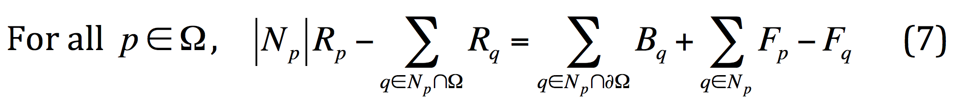
Here the neighborhood N_p is the pixel above, below, left, and right of p, Ω is the set of matted pixels (M = 1), and ∂Ω are the pixels that are not in Ω but have a neighbor in Ω. The unknowns are the result R in the matte region Ω. This equation comes from the Poisson equation (see also Discrete Poisson equation), which has many scientific applications. Thus the title "Poisson image editing" of the paper.

Your program should first count the number of unknowns n = |Ω| (which is also the number of equations). You will solve a sparse linear system of equations Au = b for the unknown pixel colors u, where A is nxn matrix and u and b are nx1 vectors. You can create the sparse matrix A using MATLAB sparse or Python scipy.sparse.lil_matrix. The entries of the matrices A and b can be set based on the left- and right-hand sides of the Equation (7), respectively. You can solve using MATLAB conjugate gradient or Python conjugate gradient. Finally, you can compute the result by copying the background B outside Ω and the appropriate pixels from u in Ω.

Notes:

We suggest to first create arrays to map between unknown variables in Equation (7) and pixel coordinates. For the forward map, you can use an 1D array that maps from the index i of an unknown variable in u to an (x, y) coordinate. For the reverse map, you can use an image that stores at each (x, y) pixel the index i of its corresponding unknown variable in u.
A next implementation step is to build the (sparse) matrix A and vector b. You can do this by looping over all matted pixels p which are the equations of (7), that is the matrix and vector row number.
Your matrix A should be symmetric, with 4s on the main diagonal and -1s or 0s off the main diagonal.
For very small masks (having only a few pixels of 1s in the mask) you can check that your matrix A is correct by converting back to a dense matrix (Python: A.todense(), MATLAB: full(A)). Do not do this for large masks or you will run out of memory.
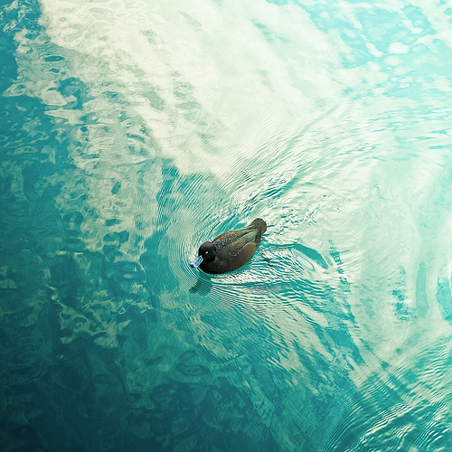
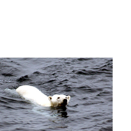
Example images: background, foreground, matte. For debugging you may wish to crop out a small region to reduce the number of variables.
As a sanity test, you can run your program on the same image for both foreground and background. This should give back the unaltered input image.

Optional part: Seam carving

The optional part is to implement seam carving which is described separately.

Policies

Feel free to collaborate on solving the problem but write your code individually.

Submission

Submit your assignment in a zip file named yourname_project2.zip. In the root directory place a README.txt file that is your writeup, which should include:

Your name
UVA computing ID
Operating system
Note any unfinished parts of the assignment, and any extra credit you did

For the required part, place a subdirectory part1 in your zip containing:

Source for your gradient domain compositing implementation.
Add to your README writeup a brief description of how to run the program.
Include the result of your gradient-domain compositing (result.png) with the provided background, foreground, and matte images. You can additionally include results on other images.

Finally submit your zip to UVA Collab.